
Predicting Sensational Stats, pt 3
Predicting Sensational Stats, pt 3
Taking a closer look at player consistency.

In our previously explained stat prediction model, we estimated player stat lines using a hierarchical Poisson regression model. We chose this model for it’s simplicity, but the trade off was that it didn’t capture the possibility that players could put up unreasonable stat lines. For example, last week Giannis scored 50 points. In 4,000 simulations of our original model, the most points Giannis ever scored in a game was 49 points.
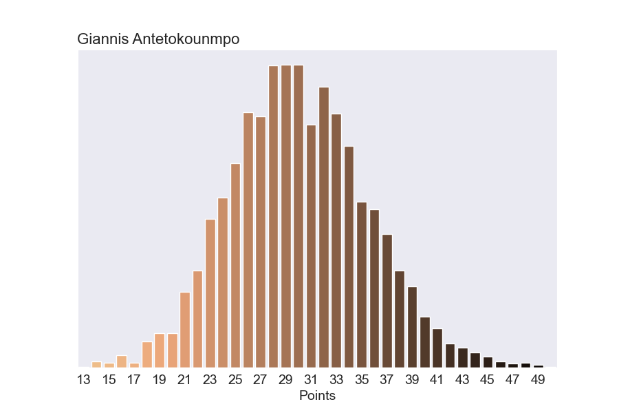
This is a well known limitation with Poisson models. So we wanted to refine our model to account for the possibility that players occasionally put up unreasonably sensational stats.
We chose to use a negative binomial model. The full details of the model are at the bottom of the post, but at a high level the model learns an additional parameter for each player that indicates how consistent that player is. If a player is extremely consistent, the chance that they’ll score 50 points in a night is very low. But if a player is wildly inconsistent, that chance is higher.
Is it better if a player is consistent or inconsistent? On one hand, a player that scores exactly 30 points every night is a reliable asset to a team. On the other hand, a player that scores 60 points every other night (and 0 points on the other nights) has the same average points per game, but is much more exciting to watch. As a fan of the sport, I’ll take inconsistency.
As always, we keep track track of how uncertain our model is about each parameter. So if we say a player is extremely consistent, we’ll know how sure the model is in that statement. And just like our Poisson model, our negative binomial model naturally handles players with limited data without any hacky rules like “limited to players with at least 19 games”.
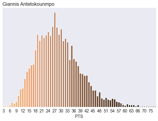
Going back to Giannis, here's our what our new model predicts he’ll score on any given night.
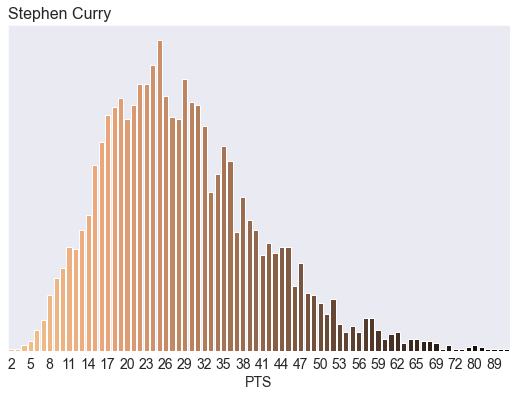
Here’s another illustrative example. Our old model never predicted Steph would score more than 55 points in a game. And practically, it put negligible probabilities on anything greater than 47 points in a game. But c’mon.

In our new model, Steph can occasionally go off:
Player Consistency Across the League
Since our model learns a value for how consistent each player is, we can get a sense of which players are consistent and which aren’t. In NBA-on-TNT-terminology: “who brings it night after night?”
In the plot below, we’re looking at how “inconsistent” a handful of players are at scoring points. Although the value has a real-life meaning related to how much variance each player is predicted to have game-to-game, it’s easiest just to think of this as Inconsistency Power Rankings.
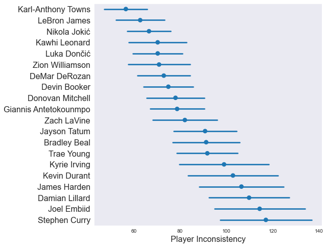
Looking at the plot above, it’s pretty easy to come up with a narrative that explains who is consistent and who isn’t.
Importantly, you need to look at the confidence intervals. On the high end (Harden, Curry, etc), the model has a hard time pinpointing exactly how inconsistent those players are. But one thing is clear: the model is certain that players near the top like LeBron and Jokic are more consistent than players near the bottom like Steph and Harden. It would be a mistake to say with certainty that Steph is more inconsistent than Embiid, but it would be reasonable to say that Kawhi is more consistent than Lillard (for example).
Looking Ahead
The model described in this post works very well at predicting all aspects of consistency. For example, which players routinely get to the free throw line? Who can you count on to turn the ball over? It could be fun to look more in depth at these types of questions.
Also, we have two posts completely written up and ready to distribute. However, the models need some more diagnosing before they’re ready to go.
Model
The model is a hierarchical negative binomial model. We also spent a good deal of time on a quasi-Poisson model, but the negative binomial sampled much faster and gave better results.
It’s worth noting that Stan has an alternative parameterize of the negative binomial distribution that makes developing models and interpreting parameters much more convenient.
data {

    int<lower=0> n_players;
    int<lower=0> n_stats;
    int stats[n_stats];
    int stats_player_index[n_stats];

}

parameters {

    // Mu terms
    vector<lower=0>[n_players] player_value;

    // Hierarchical Parameters
    real<lower=0> theta_bar;
    real<lower=0> sigma_bar;

    // Variance Terms
    vector<lower=0>[n_players] overdispersion;

}


model {

    // Hierarchical Prior on mu
    theta_bar ~ normal(0, 25);
    sigma_bar ~ cauchy(0, 5);
    player_value ~ normal(theta_bar, sigma_bar);

    //  Prior on Variance
    overdispersion ~ gamma(2, 2);


    // Negative Binomial Regression

    for (stat in 1:n_stats) {
      stats[stat] ~ neg_binomial_2(player_value[stats_player_index[stat]], overdispersion[stats_player_index[stat]]);
  }
}

generated quantities {
   int player_36_estimate[n_players];

   vector[n_players] player_variance;

   for (player in 1:n_players) {
     player_36_estimate[player] = neg_binomial_2_rng(player_value[player], overdispersion[player]);

     player_variance[player] = player_value[player] * player_value[player] / overdispersion[player];
   }

}