
Predicting Sensational Stats, pt 2
Predicting Sensational Stats, pt 2
Points, Rebounds, Blocks, Everything.

In our last post we introduced our model to predict stat lines, using assists as an illustration. In this post, we’ll dive a bit deeper into how our stat prediction model works and what it predicts.
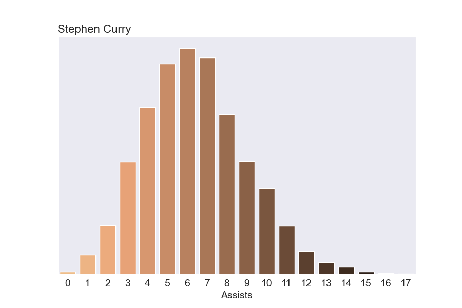
How many assists is Steph Curry going to get on a given night? Well, it varies a lot from night to night. Our model predicts somewhere between 1 and 13 assists, with 5-8 being most likely. So what’s the chance he has a mega 10+ assist night? 12.3%, not bad.
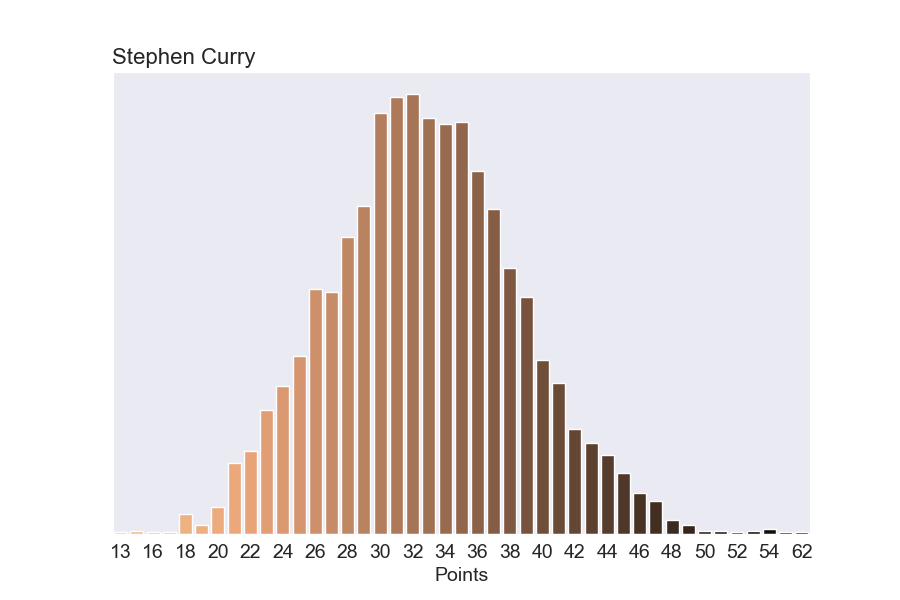
But our model for predicting sensational stats is more general than just assists. It predicts every box score counting stat. So we can also predict the chance he’ll score a ton of points. The chance he scores 45+ points on a given night is 2.8%. That means a few times a year at least he’ll go off for 45+.
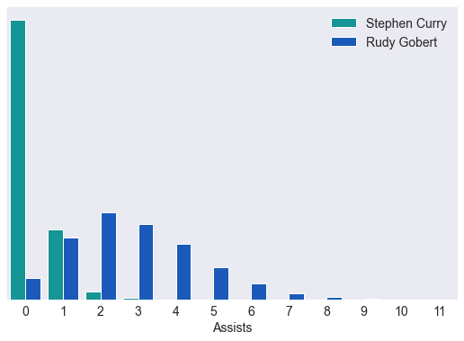
And even stats he’s not good at like blocks. There’s a less than 1% chance he’ll get 3 blocks in a night (but not impossible). That compares to Rudy Gobert who regularly gets 3+ blocks.
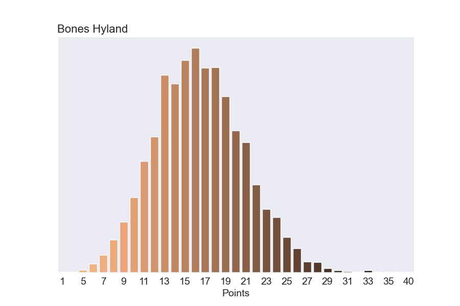
A key aspect our model is it can make good predictions even when players have little data (for example, rookies). Bones Hyland has only played 237 minutes in 15 games. But by taking advantage of how other players in the league typically perform combined with Bones stats so far, we can get predictions for how likely it would be for Bones to have a great shooting night. If Bones played 36 minutes, our model predicts a 23% chance he could score at least 20 points.
Stan Model
You can stop reading. This section is only for people curious about the underlying probability model. Either because they want to understand the details or they want to expand on it themselves. Here's our Stan model.
The model is essentially poisson regression on each player’s counting stats per game using their minutes played as an offset. It uses a hierarchical prior on the player’s parameters to facilitate learning parameters for players with little data.
I’ve evaluated these models in depth, and at some point, I need to switch them from poisson to negative binomial so I have more control over the variance. The cost of maintaining a negative binomial model might not be worth the benefit, though.
data {
    int<lower=0> n_players;
    int<lower=0> n_stats;
    int stats[n_stats];
    int stats_player_index[n_stats];
    vector[n_stats] minutes;
}

parameters {
   vector[n_players] player_value;
   real theta_bar;
   real<lower=0> sigma_bar;
}

model {
    // Hierarchical Prior
    theta_bar ~ normal(0, 10);
    sigma_bar ~ cauchy(0, 5);
    player_value ~ normal(theta_bar, sigma_bar);

    // Poisson Regression
    for (stat in 1:n_stats) {
      stats[stat] ~ poisson(exp(log(minutes[stat]) + player_value[stats_player_index[stat]])) ;
  }
}

generated quantities {
   // Stats per 36 minutes
   int player_36_estimate[n_players];
   for (player in 1:n_players) {
     player_36_estimate[player] = poisson_rng(exp(log(36) + player_value[player]));
   }
}